Week 10 - Causality I
Prof. C. Austin Davis
Spring 2025
Roadmap for today
- Quiz
- Exam review
- Presentations
- The fundamental problem of causal inference
- Randomized controlled trials
Quiz
Exam
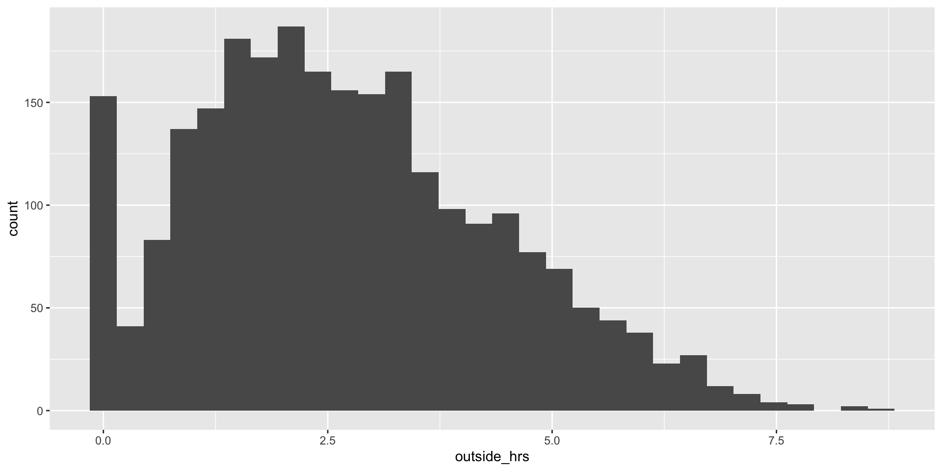
A histogram of time outside
A histogram of time outside
Ozone and health
| (1) | (2) | (3) | |
|---|---|---|---|
| (Intercept) | 0.228 *** | -0.092 *** | -0.525 *** |
| (0.009) | (0.015) | (0.017) | |
| asthma | -0.093 *** | 0.038 * | |
| (0.020) | (0.015) | ||
| ozone | 1.046 *** | 1.229 *** | |
| (0.045) | (0.036) | ||
| outside_hrs | 0.138 *** | ||
| (0.004) | |||
| *** p < 0.001; ** p < 0.01; * p < 0.05. | |||
- Each column is a regression
- Each row is an explanatory variable
Ozone and health
| (1) | (2) | (3) | |
|---|---|---|---|
| (Intercept) | 0.228 *** | -0.092 *** | -0.525 *** |
| (0.009) | (0.015) | (0.017) | |
| asthma | -0.093 *** | 0.038 * | |
| (0.020) | (0.015) | ||
| ozone | 1.046 *** | 1.229 *** | |
| (0.045) | (0.036) | ||
| outside_hrs | 0.138 *** | ||
| (0.004) | |||
| *** p < 0.001; ** p < 0.01; * p < 0.05. | |||
- Top number is estimated slope coefficient \(\hat{\beta}\)
- Number in parentheses is standard error
Ozone and health
| (1) | (2) | (3) | |
|---|---|---|---|
| (Intercept) | 0.228 *** | -0.092 *** | -0.525 *** |
| (0.009) | (0.015) | (0.017) | |
| asthma | -0.093 *** | 0.038 * | |
| (0.020) | (0.015) | ||
| ozone | 1.046 *** | 1.229 *** | |
| (0.045) | (0.036) | ||
| outside_hrs | 0.138 *** | ||
| (0.004) | |||
| *** p < 0.001; ** p < 0.01; * p < 0.05. | |||
- Asterisks or “stars” indicate rejecting the null
- Usually 0.1 is 1 star, 0.05 is 2 stars, and 0.01 is 3 stars
These regressions tell a story
How to interpret regression predictions?
- Mean or “expected” value of outcome for particular value(s) of explanatory
- Predictions or slopes help assess importance of relationship
These regressions tell a story
What is the null hypothesis?
- No true relationship between variables [in the population]
- Any apparent relationship in sample due to random chance
Rejecting the null
- Sample (\(\hat{\beta}, \text{SE}(\hat{\beta})\)) very unlikely under the null
- Compare p-value to subjective thresholds
- p-value measures strength of evidence that there is some relationship
These regressions tell a story
| (1) | (2) | (3) | |
|---|---|---|---|
| (Intercept) | 0.228 *** | -0.092 *** | -0.525 *** |
| (0.009) | (0.015) | (0.017) | |
| asthma | -0.093 *** | 0.038 * | |
| (0.020) | (0.015) | ||
| ozone | 1.046 *** | 1.229 *** | |
| (0.045) | (0.036) | ||
| outside_hrs | 0.138 *** | ||
| (0.004) | |||
| *** p < 0.001; ** p < 0.01; * p < 0.05. | |||
These regressions tell a story
Magnitude (asthma only)
- Hospitalization rate of people without asthma: \(0.228\)
- With asthma: \(0.228 + ( -0.093 ) \times 1 = 0.135\)
- Asthmatics \(9.3\) pp less likely to be hospitalized
Strength of the evidence
- test statistic of \(-4.606\), p-value of \(4.31e-06\)
- Reject the null at all conventional thresholds
- Very unlikely relationship in sample is due to random chance
These regressions tell a story
Magnitude of the relationship (asthma only)
- Hospitalization rate of people without asthma: \(0.228\)
- With asthma: \(0.228 + ( -0.093 ) \times 1 = 0.135\)
- Asthmatics \(9.3\) pp less likely to be hospitalized
These regressions tell a story
| (1) | (2) | (3) | |
|---|---|---|---|
| (Intercept) | 0.228 *** | -0.092 *** | -0.525 *** |
| (0.009) | (0.015) | (0.017) | |
| asthma | -0.093 *** | 0.038 * | |
| (0.020) | (0.015) | ||
| ozone | 1.046 *** | 1.229 *** | |
| (0.045) | (0.036) | ||
| outside_hrs | 0.138 *** | ||
| (0.004) | |||
| *** p < 0.001; ** p < 0.01; * p < 0.05. | |||
These regressions tell a story
Magnitude of the relationship (ozone only)
- What’s a good ozone level? A bad one? \[P_{10} = 0.089, P_{90} = 0.513\]
- How does hospitalization change? \[\Delta \text{Hosp} = (0.513 - 0.089) \times 1.046 = 0.444\]
These regressions tell a story
Strength of the evidence (ozone only)
- test statistic of \(23.19\), p-value \(6.54e-108\)
- Reject the null at all conventional thresholds
- Very unlikely relationship in sample is due to random chance
These regressions tell a story
| (1) | (2) | (3) | |
|---|---|---|---|
| (Intercept) | 0.228 *** | -0.092 *** | -0.525 *** |
| (0.009) | (0.015) | (0.017) | |
| asthma | -0.093 *** | 0.038 * | |
| (0.020) | (0.015) | ||
| ozone | 1.046 *** | 1.229 *** | |
| (0.045) | (0.036) | ||
| outside_hrs | 0.138 *** | ||
| (0.004) | |||
| *** p < 0.001; ** p < 0.01; * p < 0.05. | |||
These regressions tell a story
Putting it all together: adding hours outside
- \(\hat{\beta}_{\text{Hours}} = 0.138\)
- \(\hat{\beta}_{\text{Asthma}}\) changes from \(-0.093\) to \(0.038\)
- \(\hat{\beta}_{\text{Ozone}}\) increases from \(1.046\) to \(1.229\)
- All are statistically significant (at least at 0.05)
These regressions tell a story
Failing to account for hours outside leads to
- Omitted variable bias
- Overestimate of importance of asthma
- Underestimate of danger from ozone
These regressions tell a story
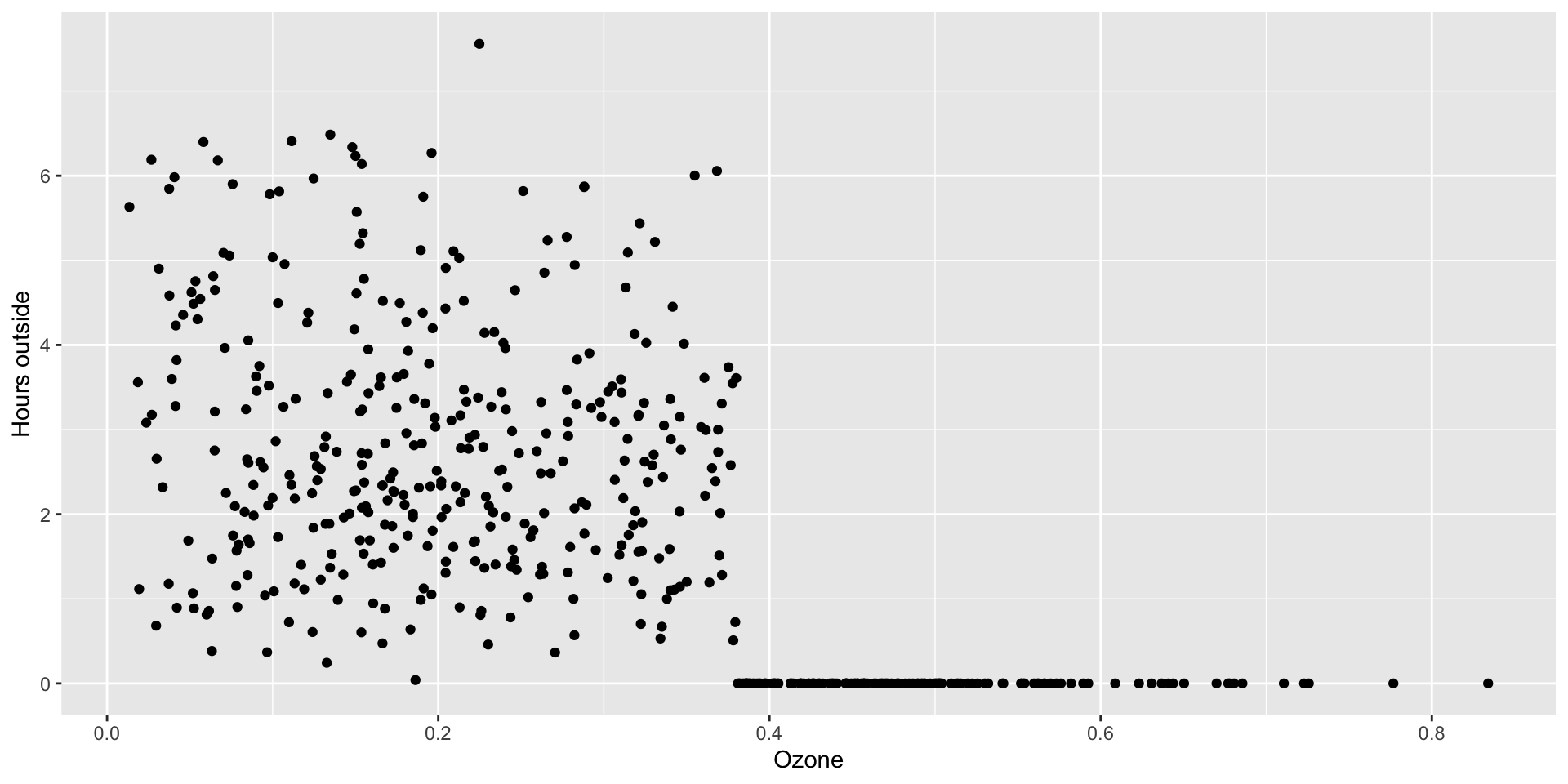
- Asthmatics engage in protective behavior
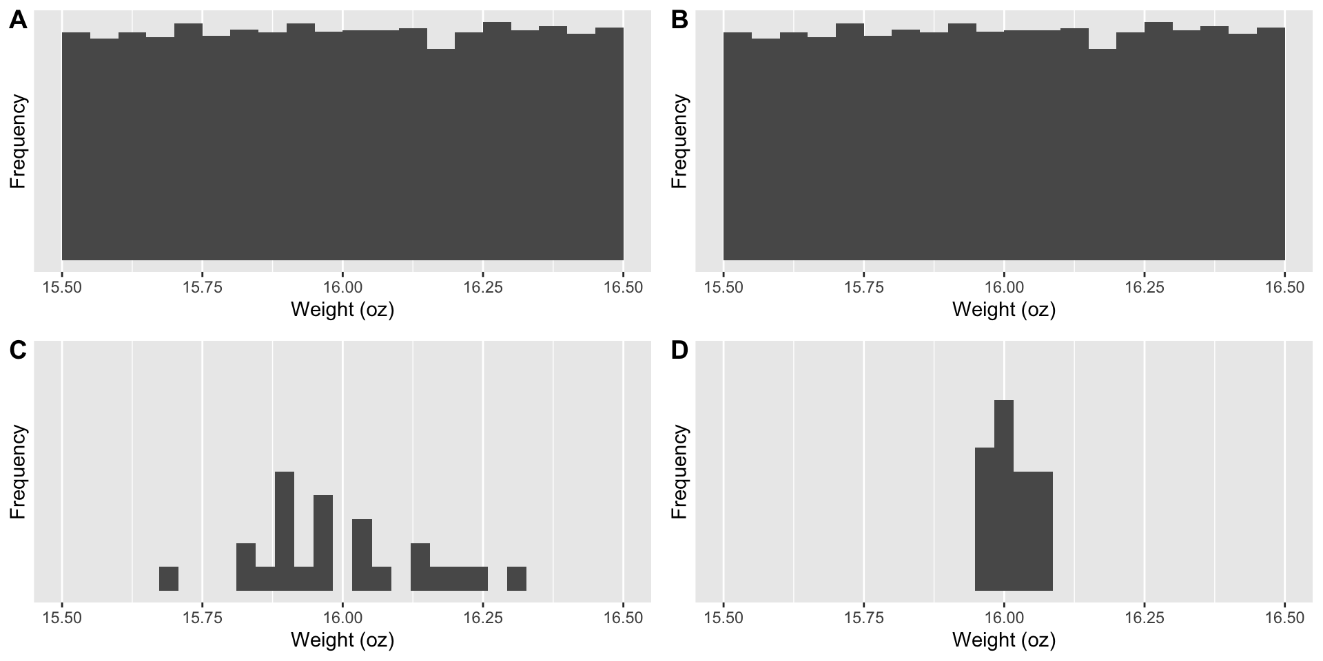
Visualizing the Central Limit Theorem
Test scores and admissions

Rejecting a true null

- Type 1 Error: asserting a relationship that isn’t there
- Mistakenly reject true null one in 20 times at 0.05
- Test enough variables or subsamples, you will find something
- Formal methods exist to correct for “multiple comparisons”
Individual research presentations
Individual presentations: Apr 14
- Five minutes, four(-ish) slides
- Research question
- Data
- Preliminary results
- (optional) descriptive statistics
- Relationship between outcome and explanatory
- Discussion and directions for group work
- Basis for group formation
Tips based on planning worksheets
- Convert categorical variables to binary
- Merging datasets
- Download and explore your data!
Categorical to binary
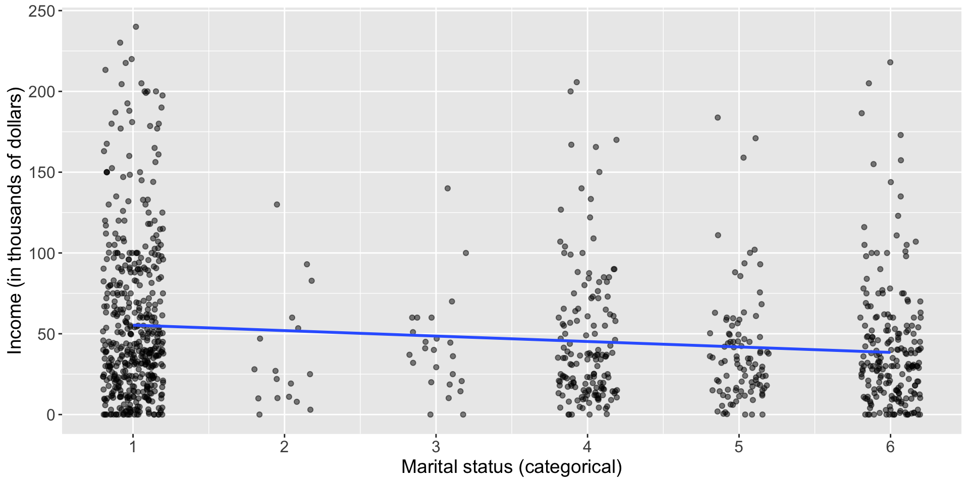
- The relationship between
- income (outcome) and
- marital status (explanatory)
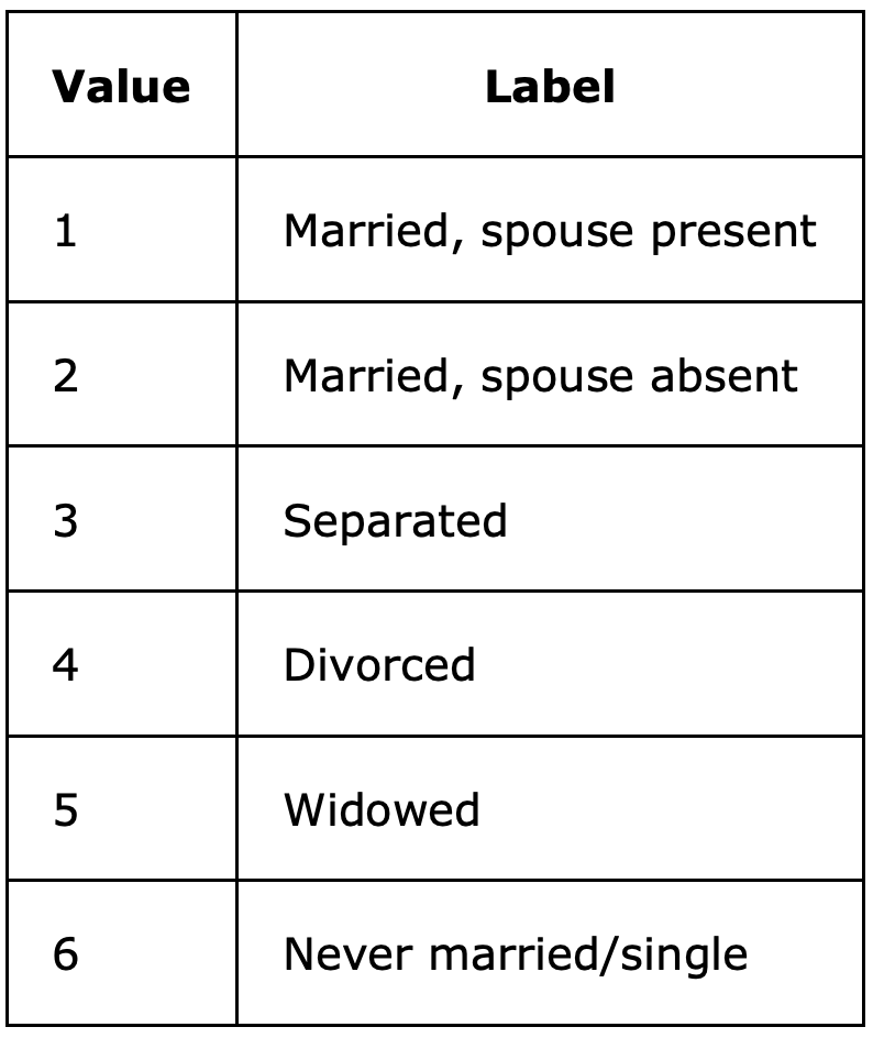
Categorical to binary
- Regression Equation: \(\text{Income} = \beta_0 + \beta_1 \times \text{Marital Status} + \varepsilon\)
| (1) | |
|---|---|
| (Intercept) | 58,691.95 *** |
| (2,440.531) | |
| MARST | -3,371.443 *** |
| (665.2156) | |
| *** p < 0.001; ** p < 0.01; * p < 0.05. | |
Categorical to binary
Categorical to binary
- Regression equation: \(\text{Income} = \beta_0 + \beta_1 \times \text{Married} + \varepsilon\)
| (1) | |
|---|---|
| (Intercept) | 41,423.6 *** |
| (2,001.686) | |
| married | 14,105.28 *** |
| (2,810.684) | |
| *** p < 0.001; ** p < 0.01; * p < 0.05. | |
Categorical to binary
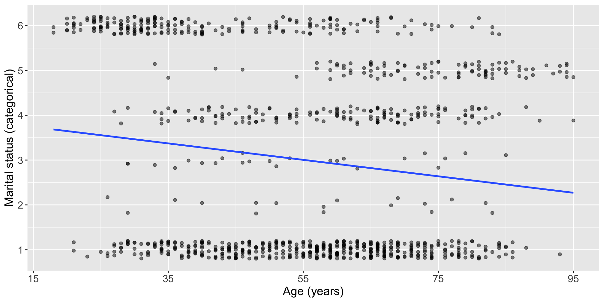
- The relationship between
- marital status (outcome) and
- age (explanatory, treat as continuous)
Categorical to binary
- Regression Equation \(\text{Marital Status} = \beta_0 + \beta_1 \times \text{Age} + \varepsilon\)
| (1) | |
|---|---|
| (Intercept) | 4.014 *** |
| (0.221) | |
| AGE | -0.018 *** |
| (0.004) | |
| *** p < 0.001; ** p < 0.01; * p < 0.05. | |
Categorical to binary
Categorical to binary
- Regression Equation \(\text{Married} = \beta_0 + \beta_1 \times \text{Age} + \varepsilon\)
| (1) | |
|---|---|
| (Intercept) | 0.415 *** |
| (0.053) | |
| AGE | 0.002 |
| (0.001) | |
| *** p < 0.001; ** p < 0.01; * p < 0.05. | |
Categorical to binary: bottom line
- OLS cannot accommodate non-binary categorical variables
- Outcome variable
- Convert to binary
- Run multiple regressions for different definitions of outcome (e.g. married vs. divorced)
Categorical to binary: bottom line
- Explanatory variable
- Convert to binary
- Include multiple binary explanatory variables to define different groups (see example in Week 6 code)
Merging datasets
- “Join” or “merge”
- Combine different variables
- Unit of observation and units must be shared
Resources
- Week 13 material
- Office hours
Get your hands dirty
- Download your data
- Open it, inspect it
- Start manipulating and analyzing in R