Week 06 - Regression with multiple explanatory variables

Prof. C. Austin Davis

Spring 2026

Roadmap for today

• Data analysis project & worksheet
• OLS recap
• At home problems
• Quiz
• DAGs and confounders
• Controlling for confounders
• Preview of next time

Data Analysis Project

Worksheet (Mar 2)

• Structure your thinking
• Get early feedback

Individual presentation (Apr 13)

• Share preliminary analysis
• Pitch your topic to classmates

Group final paper (May 4)

• Substantial expansion of preliminary analysis

Detailed instructions on Canvas

OLS Recap

What is OLS doing?

• Finding a line that minimizes SSE

What do we get out of it?

• A complete description of that line, i.e. a slope and intercept
• Big innovation over correlation: we get the slope of the line

OLS Recap

How do we read and interpret the results?

• Intercept: value of \(y\) when \(x = 0\)
• Slope: how much does \(y\) change with one unit change in \(x\)?
• Prediction: average value of \(y\) for given values of \(x\)

At-home problems

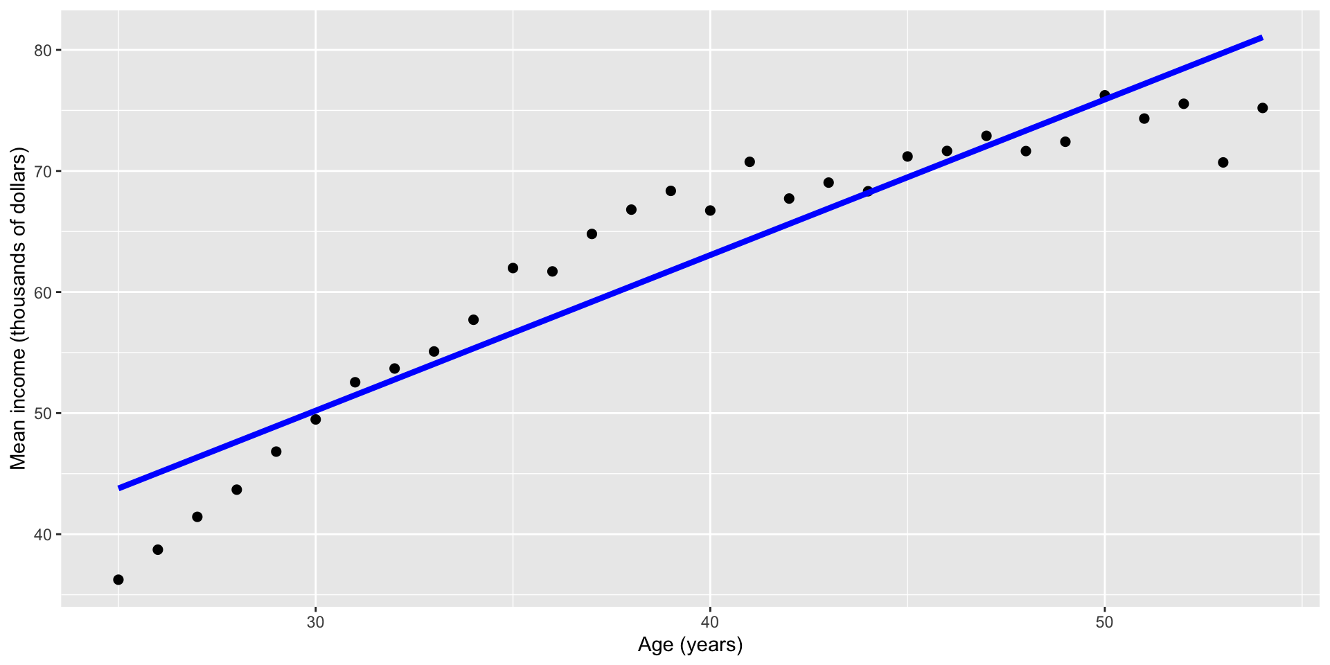
Income returns to experience

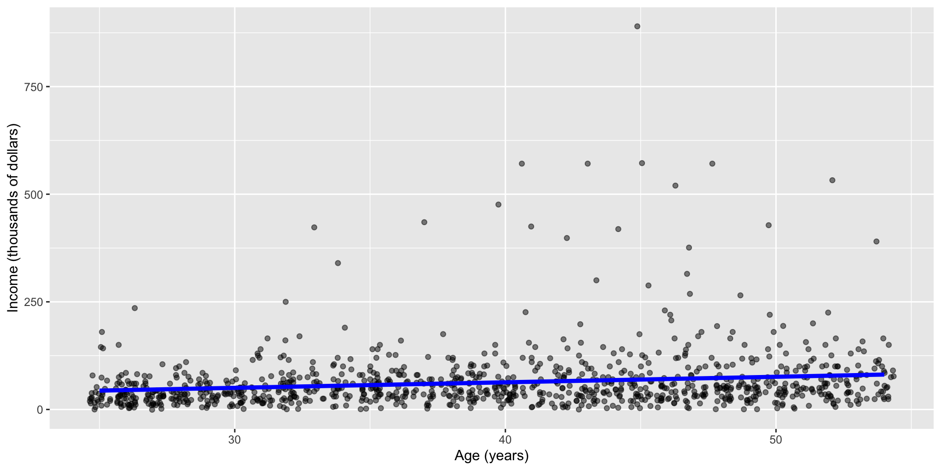
Income returns to experience

Income and young children

• OLS with binary explanatory variable: group means

Quiz

Confounding variables

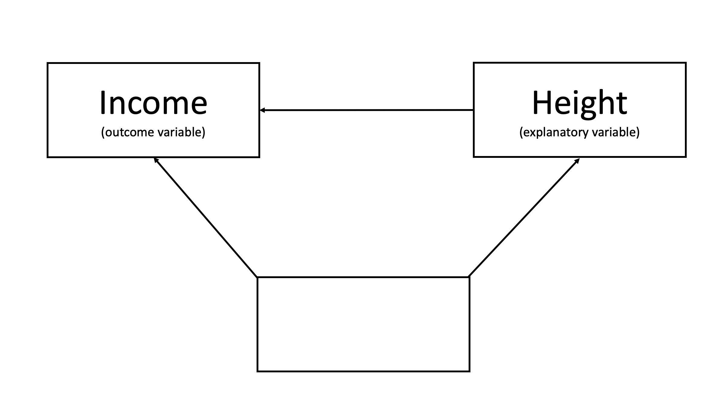
Confounding variables

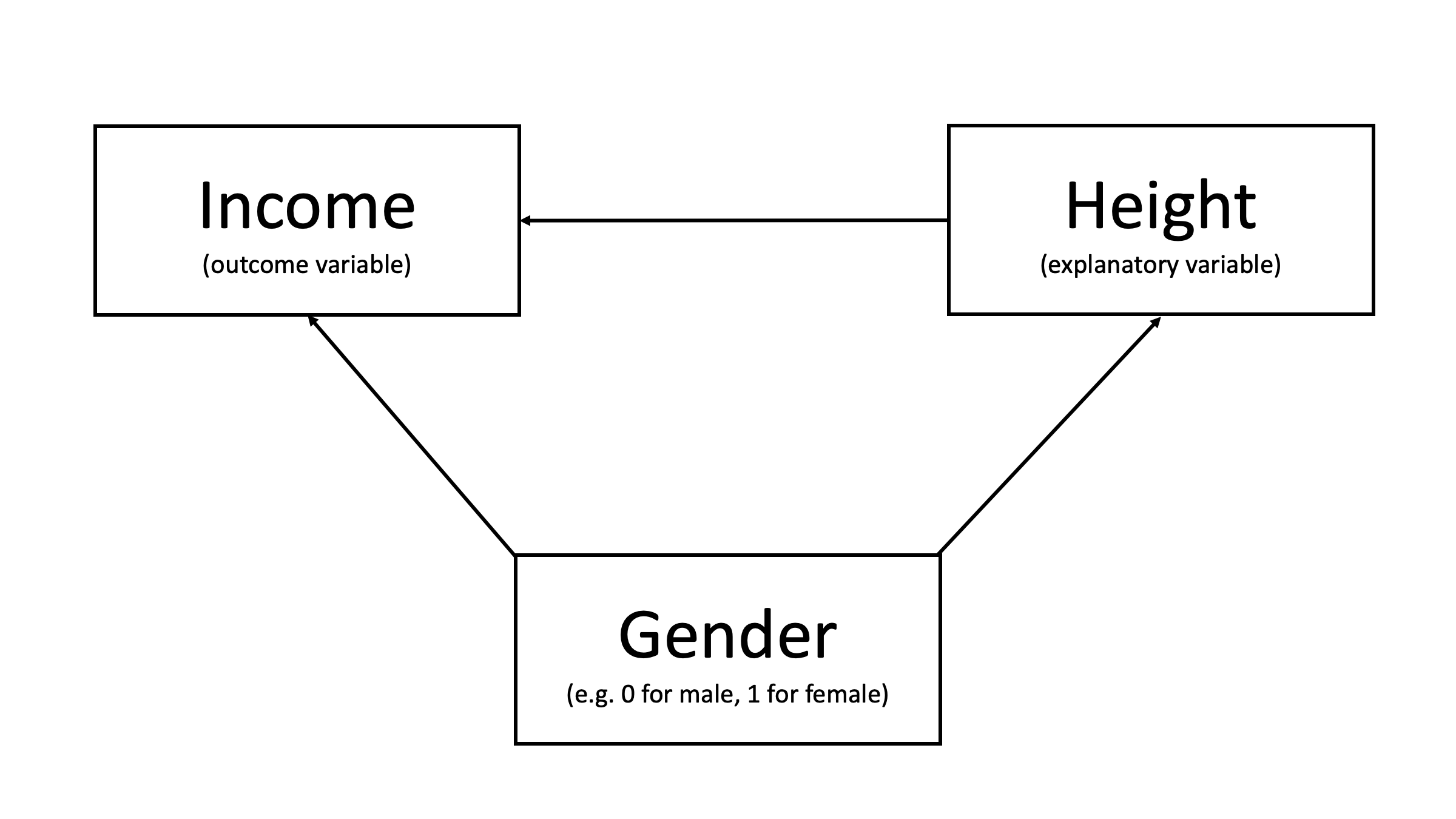
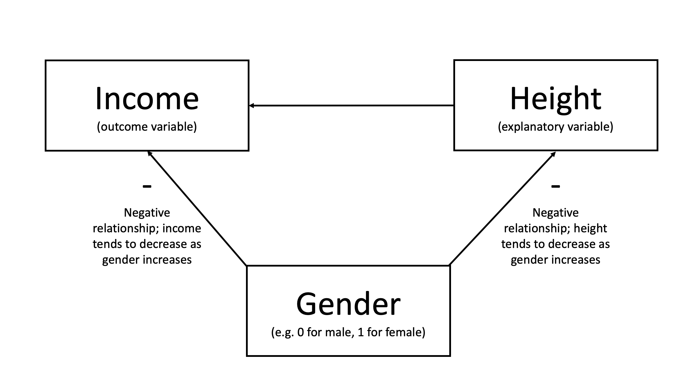
When the confounding variable increases…

If we ignore confounders, we get bias

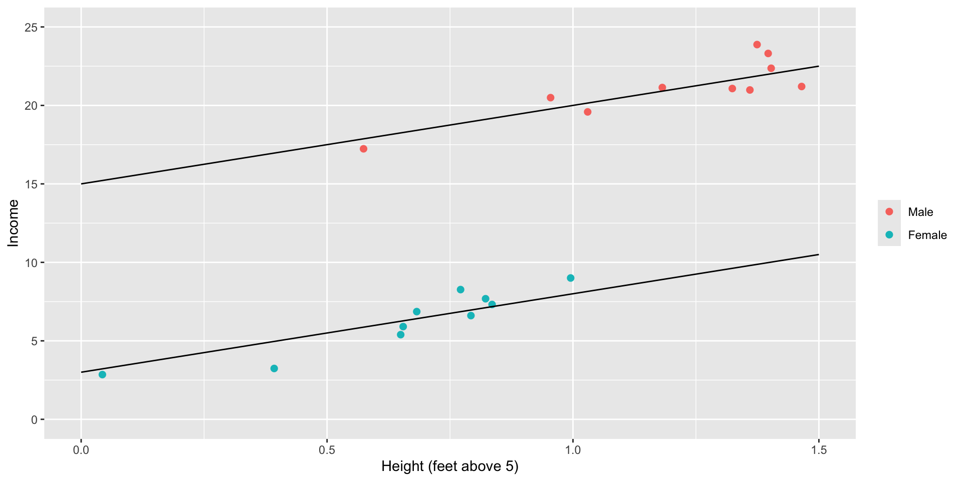
• Data would show taller people earn more because
  • of the direct causal effect AND
  • the confounding effect of gender.

If we ignore confounders, we get bias

• If our analysis omits gender and includes only height, we…
  • mistakenly attribute the effects of gender to height
  • overestimate the effect of height on income

Regression equation

\[\text{Income} = \beta_0 + \beta_1 \text{Female} + \beta_2 \text{Height} + \varepsilon\]

Estimate regression coefficients

\[\text{Income} = 15 - 12 \times \text{Female} + 0.5 \times \text{Height} + \varepsilon\]

Predicted or expected value

for a woman with \(\text{Height} = 0\)

\[\text{Income} = 15 - 12 \times 1 + 0.5 \times 0 = 3\]

Regression equation

\[\text{Income} = \beta_0 + \beta_1 \text{Female} + \beta_2 \text{Height} + \varepsilon\]

Estimate regression coefficients

\[\text{Income} = 15 - 12 \times \text{Female} + 0.5 \times \text{Height} + \varepsilon\]

Predicted or expected value

for a man with \(\text{Height} = 0\)

\[\text{Income} = 15 - 12 \times 0 + 0.5 \times 0 = 15\]

Predicted or expected value

for two women with \(\text{Height} = 66\) and \(\text{Height} = 60\)

\[\text{Income} = 15 - 12 \times 1 + 0.5 \times 66 = 36\]

\[\text{Income} = 15 - 12 \times 1 + 0.5 \times 60 = 33\]

\[\Delta \text{Income} = 0.5 \times \Delta \text{Height} = 3\]

Predicted or expected value

for two men with \(\text{Height} = 76\) and \(\text{Height} = 70\)

\[\text{Income} = 15 - 12 \times 0 + 0.5 \times 76 = 53\]

\[\text{Income} = 15 - 12 \times 0 + 0.5 \times 70 = 50\]

\[\Delta \text{Income} = 0.5 \times \Delta \text{Height} = 3\]

A tale of two intercepts

Controling for confounders

DAGs and confounders

Directed acyclic graphs

• Represent causal relationships between variables

Confounder

• Something that affects both explanatory and outcome variables

DAGs and confounders

Example: income returns to college

Strategies for handling confounders

Acknowledge

If possible, “control” for it

• Include as another explanatory variable in OLS regression

If not, work out the direction of the bias

• By leaving out the confounder, do we over- or under-estimate the relationship of interest?

Intermission

R Exercise

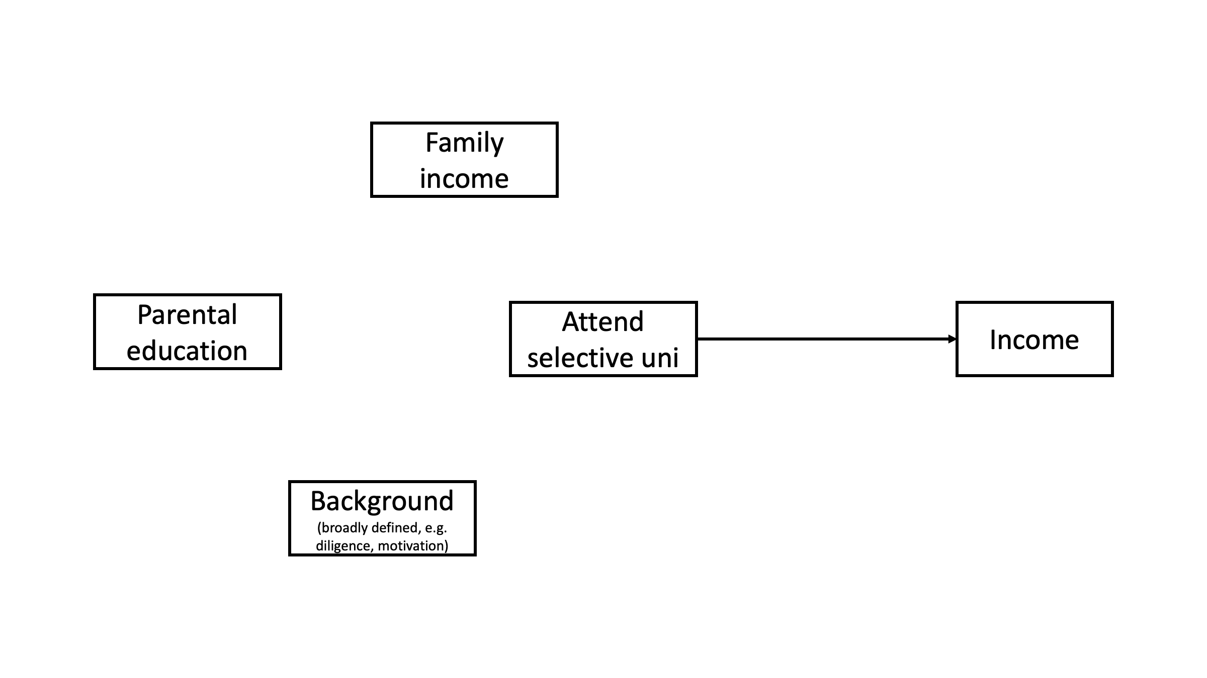
Income gains to selective (private) uni

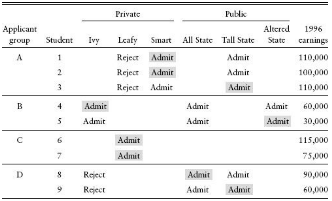
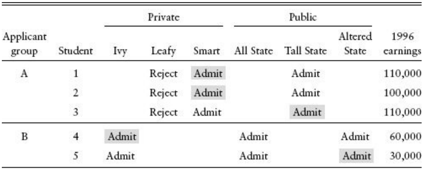
Controling for confounders

• Interest: income returns to private school
• Differences in application and admissions patterns capture
  • differences in goals or ambitions
  • differences in preparation or ability

Controling for confounders

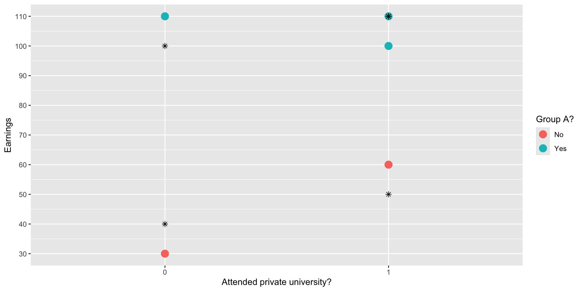
With binary explanatory variables, “expected” or “predicted” values from OLS regression are group means

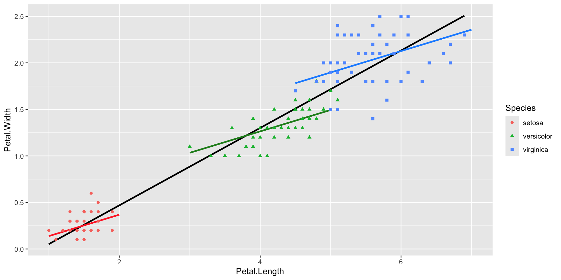
Flower power

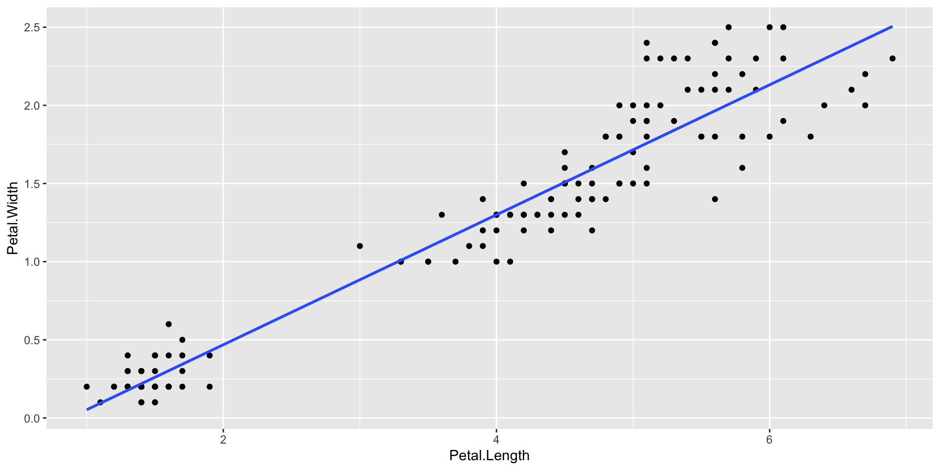
Flower power

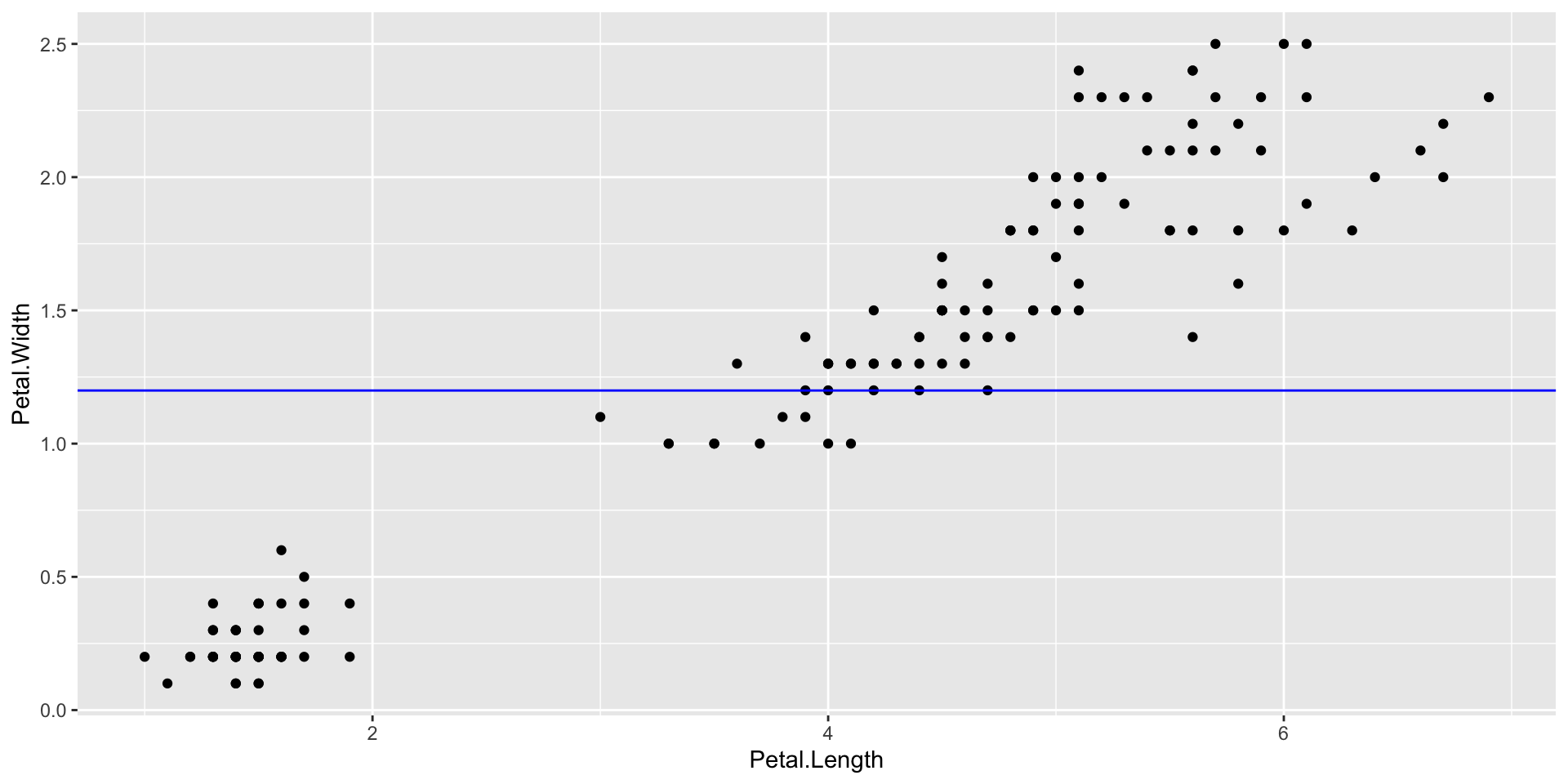
Flower power

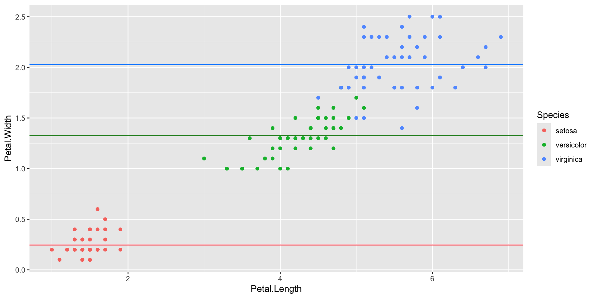
Flower power