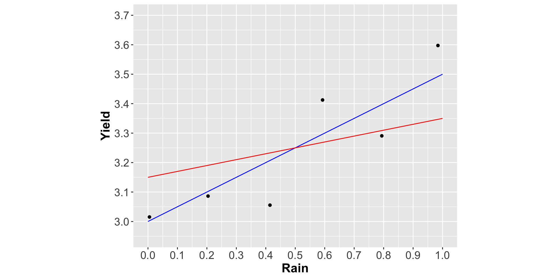
| Intercept | Slope | SSE |
|---|---|---|
| 3.00 | 0.50 | 0.06 |
| 3.15 | 0.20 | 0.14 |
| 3.15 | 0.50 | 0.21 |
| 3.00 | 0.20 | 0.27 |
| 2.96 | 0.56 | 0.06 |
Week 05 - Regression with one explanatory variable
Prof. C. Austin Davis
Spring 2025
Roadmap for today
- At home problems
- Violence in Myanmar
- Height and earnings
- Recap of variance, covariance, and correlation
- Quiz
- OLS regression with one explanatory variable
- Preview of next time
At-home problems
Fatalities in Myanmar conflict events
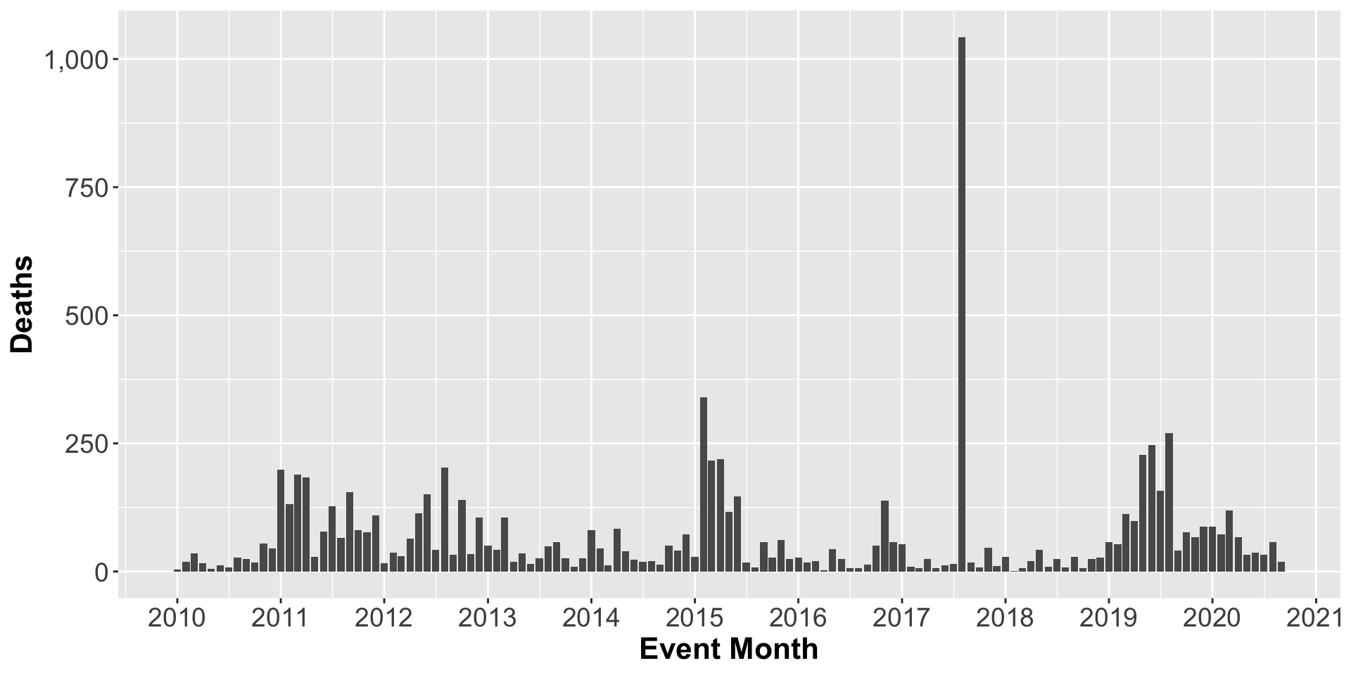
2017 Rohingya Genocide

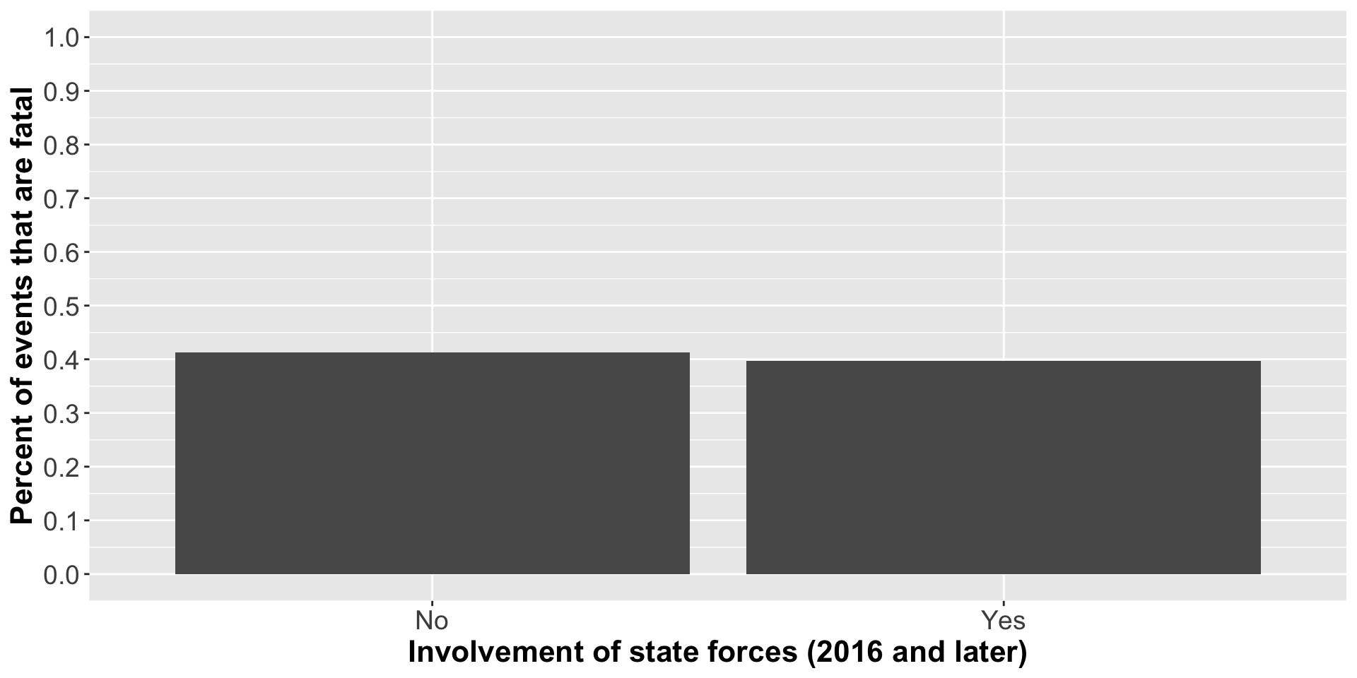
Selecting on the dependent variable
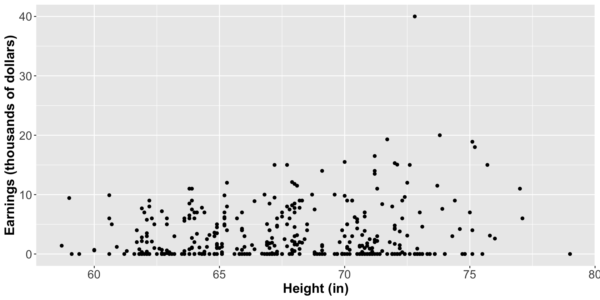
Height and earnings
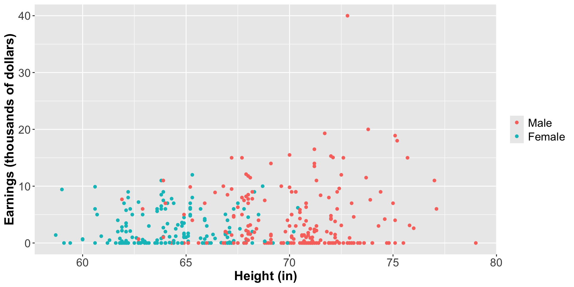
Height and earnings by gender
Recap of variance
- Measures “spread”
- \(\text{Var}(X) = \sigma^2_x = \frac{1}{N-1} \sum (x_i - \bar{x})^2\)
- how far observations deviate from mean
- Comparisons meaningful only given same units, similar mean or scale
- Why do we learn it?
- Building block for, covariance, correlation, inference
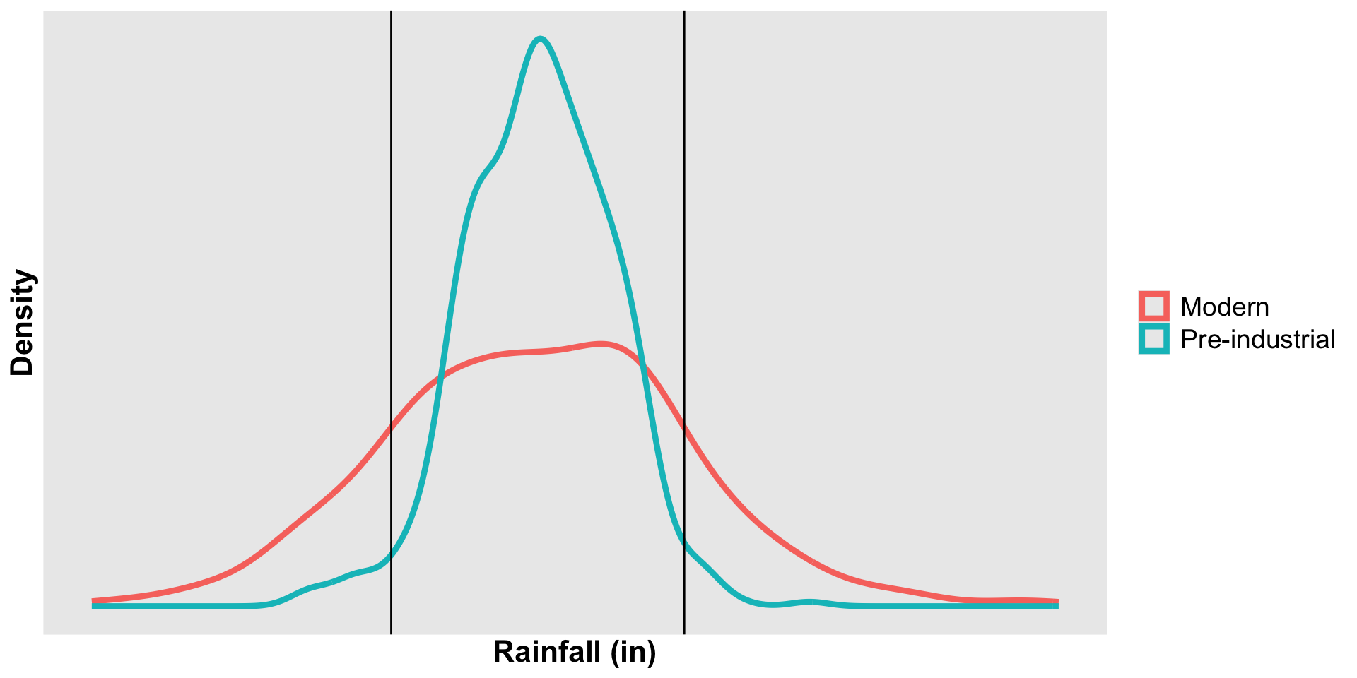
- How weird is it to see … ?
Climate change, droughts, and floods
Recap of covariance
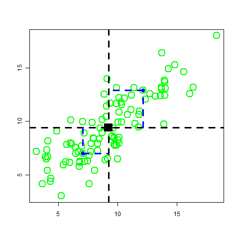
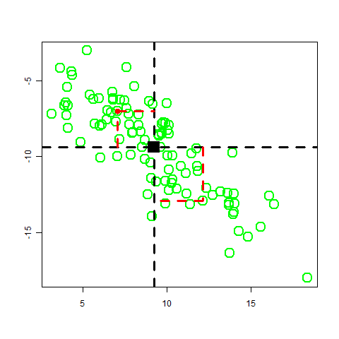
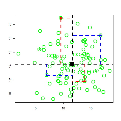
- Measures “co-movement” or relationship
- \(\text{Cov}(X,Y) = \frac{1}{N-1} \sum (x_i - \bar{x})(y_i-\bar{y})\)
- When X is above its mean, is Y above (or below) its mean?
- Definition essentially limited to straight-line relationships
Recap of covariance
- Sign is meaningful, magnitude is not
- Positive means upward-sloping relationship
- Negative means downward-sloping relationship
- Why do we learn it?
- Consistent method of identifying relationships
What does covariance look like?
What does covariance look like?
What does covariance look like?
Recap of correlation
- How close to straight-line relationship?
- \(\text{Cor}(X,Y) = \frac{\text{Cov}(X,Y)}{\sigma_x \sigma_y}\)
- Dividing by standard deviations (\(\sigma_x, \sigma_y\)) has two benefits
- Unitless number, facilitating comparison
- Bounded between -1 and 1
Recap of correlation
- Sign and magntiude are meaningful
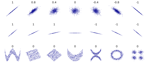
- -1 \(\Rightarrow\) all observations fall on downward-sloping line
- 0 \(\Rightarrow\) no linear relationship
- 1 \(\Rightarrow\) all observations fall on upward-sloping line
What does correlation look like?
Quiz
Ordinary least squares regression
Ordinary least squares regression
- What is it doing?
- What do we get out of it?
- How do we conduct OLS?
lm()summary()(for now)
- How do we read and interpret the results?
What is OLS doing?
What is OLS doing?
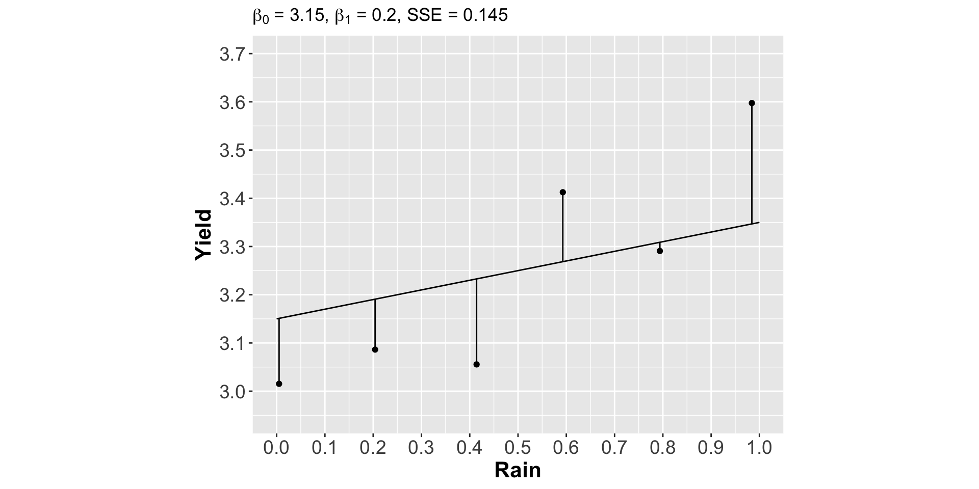
- Choosing a line that minimizes SSE
What is OLS doing?
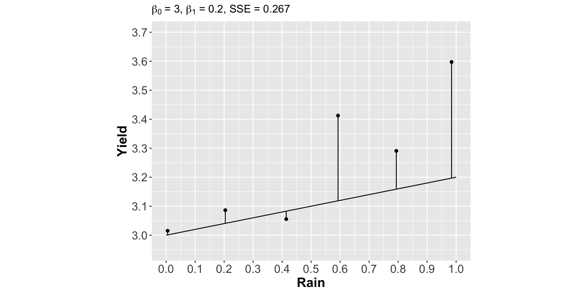
- Choosing a line that minimizes SSE
What is OLS doing?
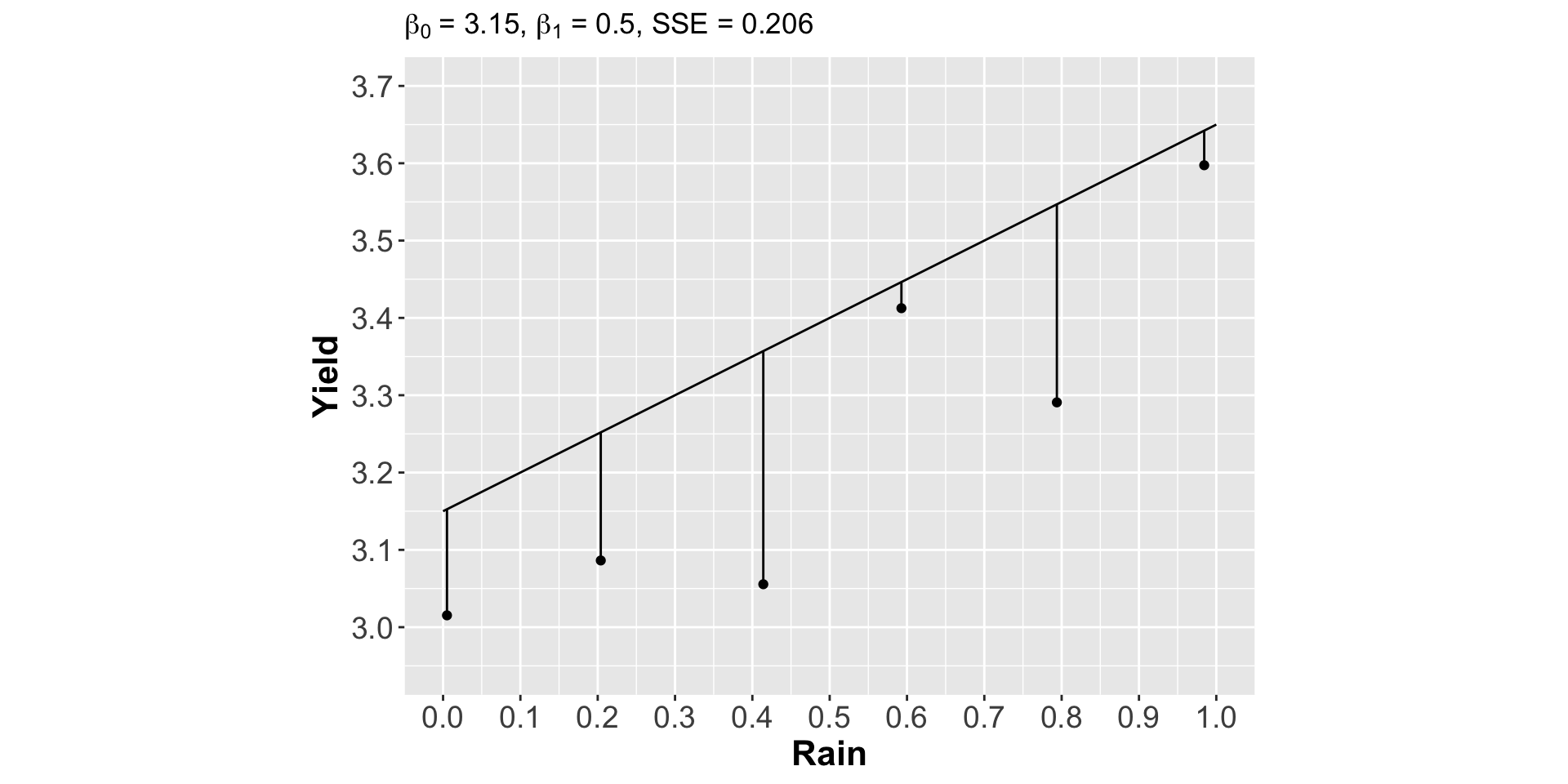
- Choosing a line that minimizes SSE
What is OLS doing?
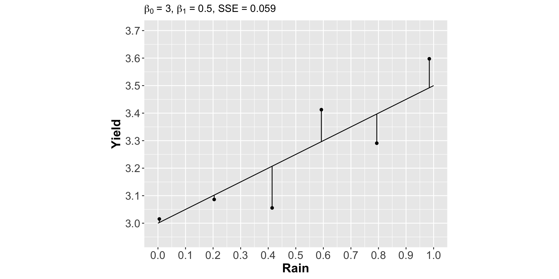
- Choosing a line that minimizes SSE
What is OLS doing?
- Choosing a line that minimizes SSE
What do we get from OLS?
- A complete description of the line: slope & intercept
- “Predicted” or “expected” values
- For a given value of explanatory variable, OLS “predicts” outcome
- Allows us to answer questions like
- If next year’s rainfall is X, what yield should we expect?
- If rainfall increases by Y, how much will yields increase?
Interpreting the slope
The “predicted” or “expected” change in the outcome variable associated with a one-unit change in the explanatory variable, i.e. if rainfall increases by one unit, how will yield change?
- How can you apply this definition to a binary (0,1) explanatory variable?
Interpreting the intercept
The “predicted” or “expected” value of the outcome variable when the explanatory variable equals zero, i.e. what are yields when there’s no rain?
- The intercept is only sometimes meaningful or interesting!
“Predicted” or “expected” values
OLS with one variable
- General equation \[\begin{aligned} \text{Outcome} &= \beta_0 + \beta_1 \times \text{Explanatory} + \varepsilon \end{aligned}\]
OLS with one variable
General equation \[\begin{aligned} \text{Outcome} &= \beta_0 + \beta_1 \times \text{Explanatory} + \varepsilon \end{aligned}\]
Using variables from quiz example \[\begin{aligned} \text{Yield} &= \beta_0 + \beta_1 \times \text{Rainfall} + \varepsilon \end{aligned}\]
OLS with one variable
General equation \[\begin{aligned} \text{Outcome} &= \beta_0 + \beta_1 \times \text{Explanatory} + \varepsilon \end{aligned}\]
Using variables from quiz example \[\begin{aligned} \text{Yield} &= \beta_0 + \beta_1 \times \text{Rainfall} + \varepsilon \end{aligned}\]
Making predictions with estimated values of \(\beta_0, \beta_1\) \[\begin{aligned} \mathbf{E}(\text{Yield}) &= 2.96 + 0.563 \times \text{Rainfall} \end{aligned}\]
OLS with one variable
- Using variables from quiz example \[\begin{aligned} \text{Yield} &= \beta_0 + \beta_1 \times \text{Rainfall} + \varepsilon \end{aligned}\]
- Making predictions with estimated values of \(\beta_0, \beta_1\) \[\begin{aligned} \mathbf{E}(\text{Yield}) &= 2.96 + 0.563 \times \text{Rainfall} \end{aligned}\]
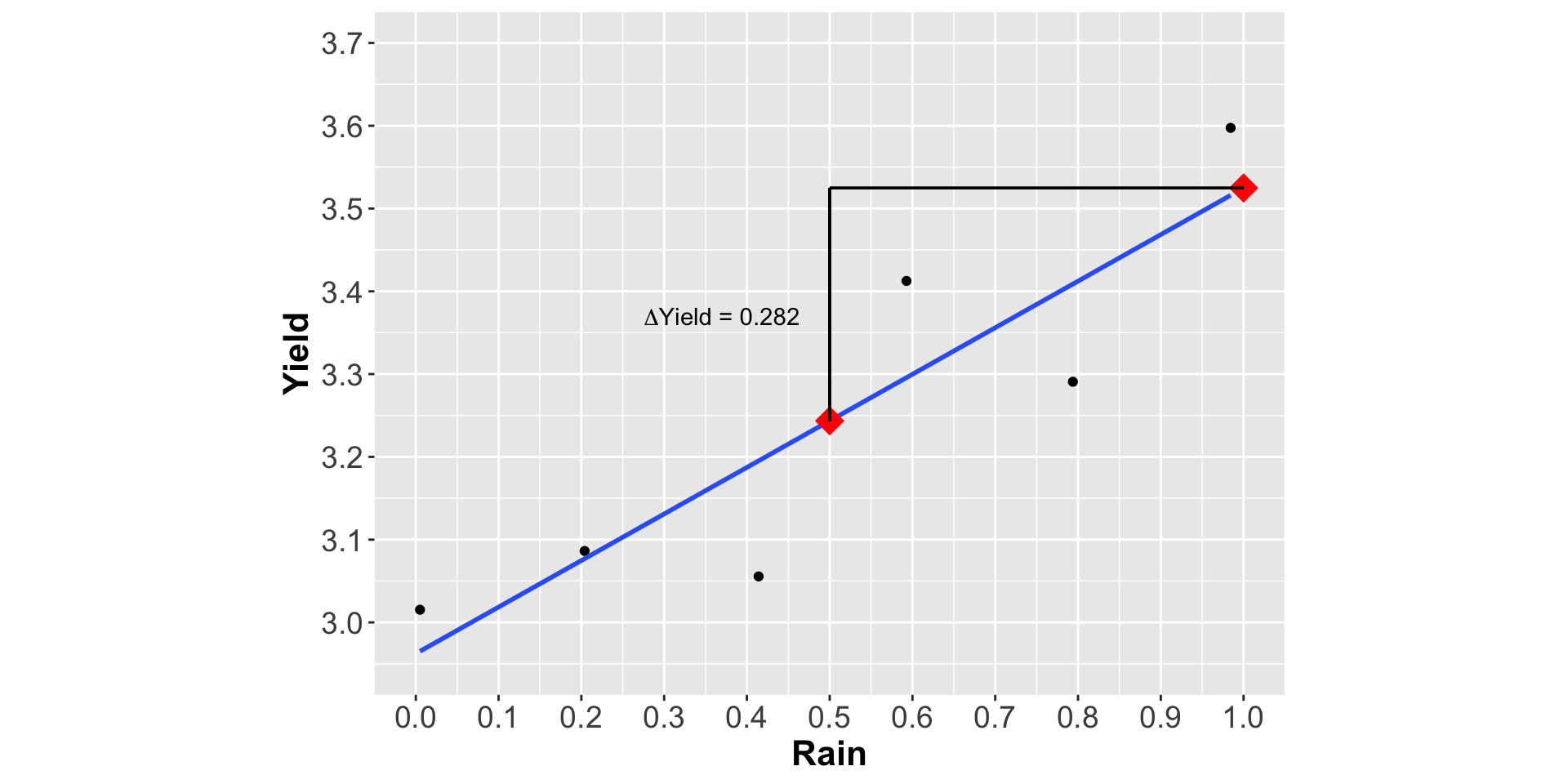
- Predicted value for a particular value of Rainfall \[\begin{aligned} \mathbf{E}(\text{Yield}) &= 2.96 + 0.563 \times 0.5 = 3.24 \end{aligned}\]
Predicting changes
- Predict yield from final value of rainfall (1.0) \[\begin{aligned} \mathbf{E}(\text{Yield}) &= 2.96 + 0.563 \times 1.0 = 3.52 \end{aligned}\]
Predicting changes
- Predict yield from final value of rainfall (1.0) \[\begin{aligned} \mathbf{E}(\text{Yield}) &= 2.96 + 0.563 \times 1.0 = 3.52 \end{aligned}\]
- Predict yield from initial value of rainfall (0.5) \[\begin{aligned} \mathbf{E}(\text{Yield}) &= 2.96 + 0.563 \times 0.5 = 3.24 \end{aligned}\]
Predicting changes
- Predict yield from final value of rainfall (1.0) \[\begin{aligned} \mathbf{E}(\text{Yield}) &= 2.96 + 0.563 \times 1.0 = 3.52 \end{aligned}\]
- Predict yield from initial value of rainfall (0.5) \[\begin{aligned} \mathbf{E}(\text{Yield}) &= 2.96 + 0.563 \times 0.5 = 3.24 \end{aligned}\]
- Take the difference \[\begin{aligned} \Delta \mathbf{E}(\text{Yield}) &= (2.96 - 2.96) + 0.563 \times (1 - 0.5) \; \; \\ = \Delta \mathbf{E}(\text{Yield}) &= (0) + 0.563 \times (0.5) = 0.282 \end{aligned}\]
Predicting changes
- Take the difference \[\begin{aligned} \Delta \mathbf{E}(\text{Yield}) &= (2.96 - 2.96) + 0.563 \times (1 - 0.5) \; \; \\ = \Delta \mathbf{E}(\text{Yield}) &= (0) + 0.563 \times (0.5) = 0.282 \end{aligned}\]
- A simple formula for changes \[\begin{aligned} \Delta \mathbf{E}(\text{Outcome}) &= \beta_1 \times \Delta \text{Explanatory} \; \; \end{aligned}\]
Visualizing predicted values
OLS Regression in R
Basic formula
[NEW OBJECT] <- lm(data = [OBJECT NAME], formula = [OUTCOME] ~ [EXPLANATORY]
- e.g.
rain_yield_ols <- lm(data = rain_yield, formula = Yield ~ Rain)
Printing results to the console
summary([OBJECT NAME]), e.g. summary(rain_yield_ols)
Preview of next time
Regression with multiple explanatory variables
Questions to ponder
How would the relationship between height and earnings change if we accounted for gender somehow in the same analysis?